Series对象
pandas库的Series对象用来表示一维数据结构,跟数组类似,但多了一些额外的功能,它的内部结构很简单(如下表),由两个相互关联的数组组成,其中主数组用于存放数据(Numpy任意类型数据)。主数组的每个元素都有一个与之相关联的标签,这些标签存储的另一个叫做Index的数组中。
|Series| -|- index|value 0|12 1|-4 2|7 3|9
In:
s = pd.Series([12,-4,7,9]) |
out:
0 12 |
可以看出左侧Index是一列标签,右侧是标签对应的元素
声明Series时,若不指定标签,pandas默认使用从0开始一次递增的数值作为标签。这种情况下,标签与Series对象中的元素索引一致。但是最好使用有意义的标签,用以区分和识别每个元素
in:
s = pd.Series([12,-4,7,9],index=['a','b','c','d']) |
out:
a 12 |
获取元素
s.values |
array([12, -4, 7, 9], dtype=int64)
s.index |
Index([‘a’, ‘b’, ‘c’, ‘d’], dtype=’object’)
s[2] |
- 7
s['c'] |
- 7
in:
s[:2] |
out:
a 12 |
in:
s[['b','c']] |
out:
b -4 |
为元素赋值
in:
s[1]=0 |
out:
a 12 |
in:
s['b'] = 1 |
out:
a 12 |
用Numpy数组或其他Series对象定义新Series对象
in:
a = np.array([1,2,3,4]) |
out:
0 1 |
in:
c= pd.Series(b) |
out:
0 1 |
这样做时不要忘记新Series对象中的元素不是原Num数组或Series对象的副本,而是对他们的引用,也就是说,这些对象是动态插入到新Series对象中。如改变原有对象元素的值,新Series对象中这些元素也会发生改变。
in:
b[2]=11 |
out:
0 1 |
in:
c |
out:
0 1 |
筛选元素
pandas库的开发是以NumPy库为基础的,因此就数据结构而言,NumPy数组的多种操作方法得以扩展到Series对象中,其中就是根据条件筛选数据结构中的元素之一方法。
in:
s[s>8] |
out:
a 12 |
运算和数学函数
适用于NumPy数组的运算符(+,-,* ,/ )或其他数学函数,也适用于Series对象。
in:
s / 2 |
out:
a 6.0 |
in:
s |
out:
a 12 |
NumPy库的数学函数,必须制定他们出处np,并把Series实例作为参数传入。
in:
np.log(s) |
out:
a 2.484907 |
Series对象的组成元素
in:
color = pd.Series([1,0,2,1,2,3],index=['white','white','blue','green','green','yellow']) |
out:
white 1 |
color.unique() |
array([1, 0, 2, 3], dtype=int64)
返回一个数组,包含去重后的元素,但乱序
in:
color.value_counts() |
out:
2 2 |
返回各个不同的元素,还计算每个元素在Series中出现次数
in:
color.isin([0,3]) |
out:
white False |
判断给定的一列元素是否包含在数据结构中,返回布尔值
in:
color[color.isin([0,3])] |
out:
white 0 |
NaN
in:
s = pd.Series([1,2,np.NaN,14]) |
out:
0 1.0 |
in:
s.isnull() |
out:
0 False |
in:
s.notnull() |
out:
0 True |
in:
s[s.notnull()] |
out:
0 1.0 |
in:
s[s.isnull()] |
out:
2 NaN |
Series用作字典
in:
mydict = {'red':2000,'blue':1000,'yellow':500,'orange':1000} |
out:
blue 1000 |
索引数组用字典的键来填充,每个索引所对应的元素为用作索引的键在字典中对应的值。你还可以单独制定索引,pandas会控制字典的键和数组索引标签之间的相关性。如遇缺失值处,pandas就会为其添加NaN。
in:
colors = ['red','yellow','orange','blue','green'] |
out:
red 2000.0 |
Series 对象之间的运算
in:
mydict = {'red':200,'blue':100,'yellow':50,'orange':100,'black':700} |
out:
black 700 |
in:
myseries + myseries2 |
out:
black NaN |
DataFrame对象
DataFrame这种列表式数据结构跟工作表(最常见的是Excel工作表)极为相似,其设计初衷是将Series的使用场景由一维扩展到多维。DataFrame由按一定顺序排列的多列数据组成,各列数据类型可以有不同。
定义DataFrame对象
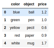
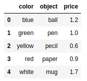
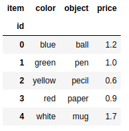
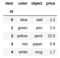
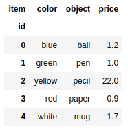
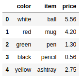
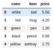
data = {'color':['blue','green','yellow','red','white'],'object':['ball','pen','pecil','paper','mug'],'price':[1.2,1.0,0.6,0.9,1.7]} |
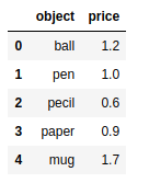
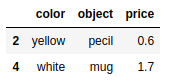
如果用来创建DataFrame对象的dict对象包含一些用不到的数据,你可以只选择自己感兴趣的。在DataFrame构造函数中,用columns选项制定需要的列即可。新建的DataFrame各列顺序与你制定的列顺序一致,而与他们在字典中的顺序无关。
frame2 = pd.DataFrame(data,columns=['object','price']) |
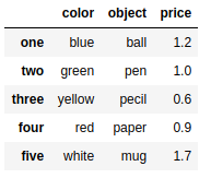
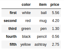
DataFrame对象和Series一样,如果Index数组没有明确制定标签,pandas也会自动为其添加一列从0开始的数值作为索引。如果想用标签作为DataFrame的索引,则要把标签放在数组中,赋给index选项
frame3 = pd.DataFrame(data,index=['one','two','three','four','five']) |
选取元素
frame.columns #列名 |
Index([‘color’, ‘object’, ‘price’], dtype=’object’)
frame.index #索引 |
RangeIndex(start=0, stop=5, step=1)
frame.values #所有元素 |
out:
array([['blue', 'ball', 1.2], |
in:
frame['price'] |
out:
0 1.2 |
in:
frame.price |
out:
0 1.2 |
in:
frame.ix[2] |
out:
color yellow |
frame |
in:
frame.loc[2] |
out:
color yellow |
in:
frame.iloc[2] |
out:
color yellow |
frame.loc[[2,4]] |
frame.iloc[[2,4]] #i表示整数 |
frame3.loc['one'] |
out:
color blue |
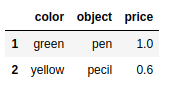
frame[1:3] |
frame['object'][3] |
‘paper’
赋值
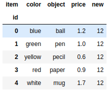
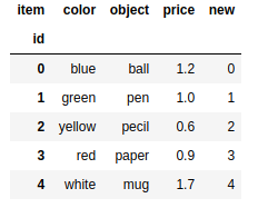
frame.index.name = 'id' |
frame['new'] = 12 |
frame['new'] = [3.0,1.3,2.2,0.8,1.1] |

in:
ser = pd.Series(np.arange(5)) |
out:
0 0 |
frame['new'] = ser |
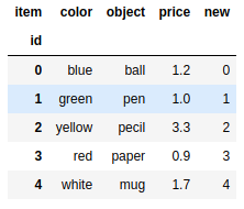
frame['price'][2] = 3.3 |
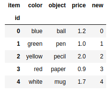
frame.set_value(2,'price',2) |
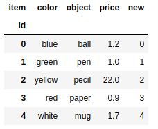
frame.at[2,'price']=22 |
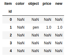
frame.isin([1.0,'pen']) |
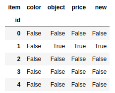
frame[frame.isin([1.0,'pen'])] |
del frame['new'] |
删除一列
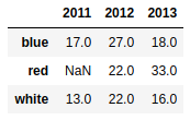
d1 = {'red':{2012:22,2013:33},'white':{2011:13,2012:22,2013:16},'blue':{2011:17,2012:27,2013:18}} |
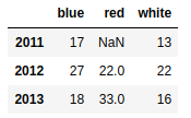
frame2.T |
Index对象
in:
ins = pd.Series([5,0,3,8,4],index=['red','blue','yellow','white','green']) |
out:
red 5 |
ins.index |
Index([‘red’, ‘blue’, ‘yellow’, ‘white’, ‘green’], dtype=’object’)
ins.idxmin() #返回索引值最小的元素 |
‘blue’
ins.idxmax() #返回索引值最大的元素 |
‘white’
重复标签的Index
serd = pd.Series(range(6),index=['white','white','blue','green','green','yellow']) |
out:
white 0 |
in:
serd['white'] |
out:
white 0 |
serd.index.is_unique |
False
判断是否存在重复项
frame.index.is_unique |
True
frame |
索引对象的其他功能
更换索引
ser = pd.Series([2,3,4,5],index=['one','two','three','four']) |
out:
one 2 |
in:
ser.reindex(['three','four','five','one']) |
out:
three 4.0 |
自动编制索引
ser2 = pd.Series([1,5,6,3],index =[0,3,5,6]) |
out:
0 1 |
in:
ser2.reindex(range(6),method='ffill') #插值,以得到一个完整的序列(前插) |
out:
0 1 |
in:
ser2.reindex(range(6),method='bfill') #插值,以得到一个完整的序列(后插) |
out:
0 1 |
删除
pandas提供专门的删除操作函数:drop()
ser3 = pd.Series(np.arange(4.),index=['red','blue','yellow','white']) |
out:
red 0.0 |
in:
ser3.drop('yellow') |
out:
red 0.0 |
in:
ser3.drop(['blue','white']) |
out:
red 0.0 |
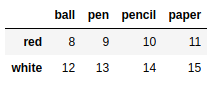
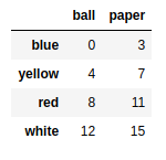
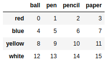
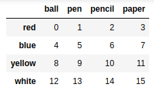
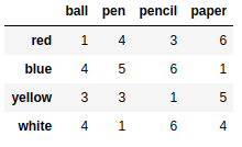
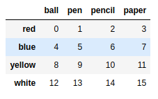
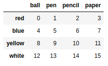
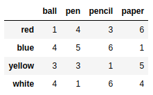
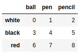
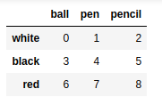
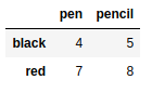
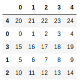
frame = pd.DataFrame(np.arange(16).reshape((4,4)),index=['blue','yellow','red','white'],columns=['ball','pen','pencil','paper']) |
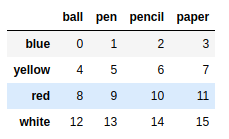
frame.drop(['blue','yellow']) #默认删除行 |
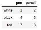
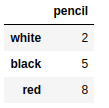
frame.drop(['pen','pencil'],axis=1) #删除列 |
add() sub() div() mul()
in:
ser4 = pd.Series(np.arange(4.),index=['red','blue','yellow','white']) |
out:
red 0.0 |
in:
ser5 = pd.Series(np.arange(5.),index=['red','blue','black','brown','yellow']) |
out:
red 0.0 |
in:
ser4 + ser5 |
out:
black NaN |
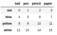
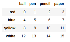
frame1 = pd.DataFrame(np.arange(16).reshape((4,4)),index=['red','blue','yellow','white'],columns=['ball','pen','pencil','paper']) |
frame2 = pd.DataFrame(np.arange(12).reshape((4,3)),index=['blue','green','white','yellow'],columns=['mug','pen','ball']) |
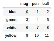
frame1 + frame2 |
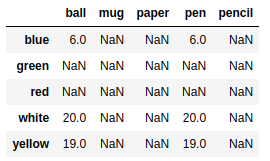
frame1.add(frame2) |
frame2 = pd.DataFrame(np.arange(16).reshape((4,4)),index=['red','blue','yellow','white'],columns=['ball','pen','pencil','paper']) |
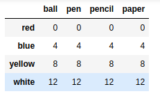
ser1 = pd.Series(np.arange(4),index=['ball','pen','pencil','paper']) |
out:
ball 0 |
frame2 - ser1 |
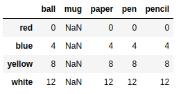
ser1['mug'] = 9 |
out:
ball 0 |
frame2 - ser1 |
通用函数
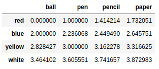
np.sqrt(frame2) #平方根 |
按行或列执行操作的函数
f = lambda x:x.max() - x.min() |
out:
ball 12 |
in:
frame2.apply(f,axis = 1) # 行 |
out:
red 3 |
in:
def f(x): |

统计函数
frame2.sum() |
out:
ball 24 |
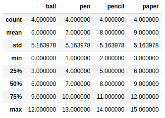
in:
frame.describe() |
排序
根据索引排序
ser = pd.Series([5,0,3,8,4],index=['red','blue','yellow','white','green']) |
out:
red 5 |
in:
ser.sort_index() #a-zp升序 |
out:
blue 0 |
in:
ser.sort_index(ascending=False) #降序 |
out:
yellow 3 |
in:
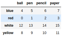
frame2 |
frame2.sort_index() |
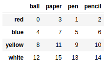
frame2.sort_index(axis=1) |
根据对象排序
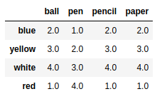
frame2.sort_values(by = 'pen') |
frame2.at['red','pen']=18 |
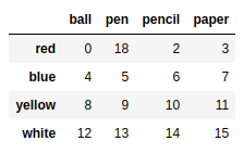
frame2.sort_values(by = 'pen') |

排位
in:
ser.rank() #排位 |
out:
red 4.0 |
in:
ser.rank(method = 'first') |
out:
red 4.0 |
in:
ser.rank(ascending=False) #降序 |
out:
red 2.0 |
in:
frame2.rank() |
frame3 = frame2.sort_values(by = 'pen') |
相关性和协方差
seq2 = pd.Series([3,4,3,4,5,4,3,2],['2006','2007','2008','2009','2010','2011','2012','2013']) |
out:
2006 3 |
seq = pd.Series([1,2,3,4,4,3,2,1],['2006','2007','2008','2009','2010','2011','2012','2013']) |
out:
2006 1 |
in:
seq.corr(seq2) |
0.7745966692414835
seq.cov(seq2) |
0.8571428571428571
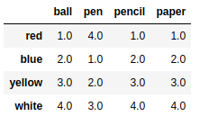
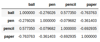
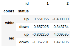
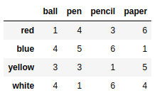
frame2 = pd.DataFrame([[1,4,3,6],[4,5,6,1],[3,3,1,5],[4,1,6,4]],index=['red','blue','yellow','white'],columns = ['ball','pen','pencil','paper']) |
frame2.corr() |
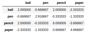
frame2.cov() |
corrwith()方法可以计算DataFrame对象的列或行与Series对象或其他DataFrame对象元素两两之间的相关性
frame2.corrwith(ser) |
out:
ball -0.140028 |
in:
f1 = frame2.corrwith(frame) |
out:
ball -0.182574 |
in:
f1.dropna() #删除NaN |
out:
ball -0.182574 |
in:
f1[f1.notnull()] |
out:
ball -0.182574 |
in:
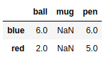
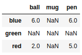
frame3 = pd.DataFrame([[6,np.nan,6],[np.nan,np.nan,np.nan],[2,np.nan,5]],index = ['blue','green','red'],columns = ['ball','mug','pen']) |
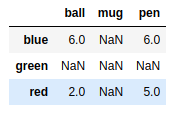
frame3.dropna() |
frame3.dropna(how ='all') |
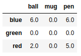
frame3.fillna(0) #指定缺失值填充 |
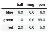
frame3.fillna({'ball':1,'mug':0,'pen':99}) |
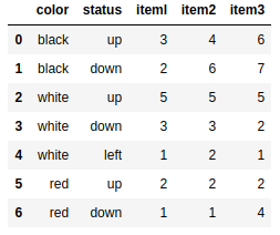
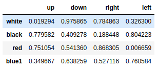
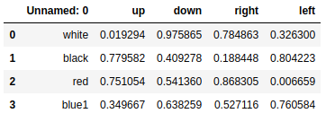
mser = pd.Series(np.random.rand(8),index=[['white','white','white','blue','blue','red','red','red'],['up','down','right','up','down','up','down','left']]) |
out:
white up 0.096961 |
in:
mser.index |
out:
MultiIndex(levels=[['blue', 'red', 'white'], ['down', 'left', 'right', 'up']], |
in:
mser['white'] |
out:
up 0.096961 |
in:
mser[:,'up'] |
out:
white 0.096961 |
mser['white','up'] |
0.09696136257353527
frame = mser.unstack() #把等级索引Series转换成简单的DataFrame对象 |
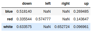
frame.stack() |
out:
blue down 0.518140 |
mframe = pd.DataFrame(np.random.randn(16).reshape(4,4), |
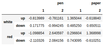
mframe.columns.names =['objects','id'] |
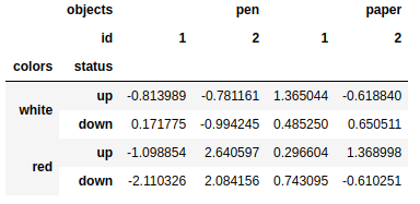
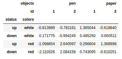
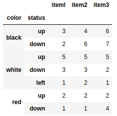
mframe.swaplevel('colors','status') #互换位置 |
mframe.sort_index(level='colors') #根据层级排序 |
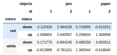
mframe.sum(level='colors') #按照层级统计 |

mframe.sum(level='id',axis=1) #按照层级统计 |
pandas:数据读写
csv和文本文件
多年以来,人们已习惯于文本文件的读写,特别是列表形式的数据。如果文件每一行的多 个元素是用逗号隔开的,则这种格式叫作CSV,这可能是最广为人知和最受欢迎的格式。
其他由空格或制表符分隔的列表数据通常存储在各种类型的文本文件中(扩展名一般 为.txt )。
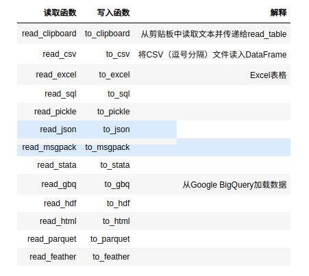
因此这种文件类型是最常见的数据源,它易于转录和解释。pandas的下列函数专门用来处理 这种文件类型:
- read_csv
- read_table
- to_csv
csvframe = pd.read_csv('myCSV_01.csv') |
csvframe = pd.read_table('myCSV_01.csv',sep=',') |
第一行作为列名称,但是往往很多数据第一行不是列名
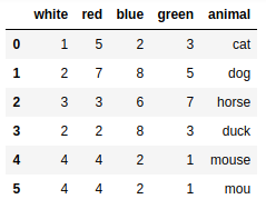
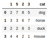
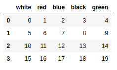
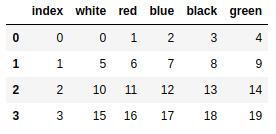
csvframe = pd.read_csv('myCSV_02.csv') |
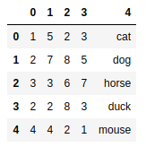
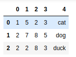
csvframe = pd.read_csv('myCSV_02.csv',header=None) #添加默认表头 |
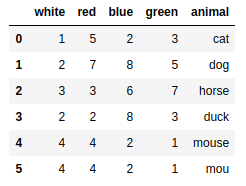
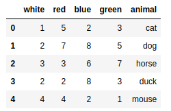
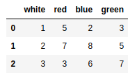
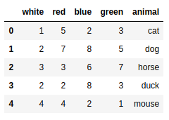
csvframe = pd.read_csv('myCSV_02.csv',names=['white','red','blue','green','animal']) #指定表头 |
csvframe = pd.read_csv('myCSV_03.csv') |
csvframe = pd.read_csv('myCSV_03.csv',index_col=['color','status']) #等级索引 |
pd.read_table('ch05_04.txt',sep='\s+') #根据正则解析 |
pd.read_table('ch05_05.txt',sep=r'\D+',header=None,engine='python') |
另一种很常见的情况是,解析数据时把空行排除在外。文件中的表头或没有必要的注释,有时用不到。使用skiprows选项,可以排除多余的行。把要排除的行的行号放到数组中,赋给该选项即可。
pd.read_table('ch05_06.txt',sep=',',skiprows=[0,1,3,6]) |
从TXT文件读取部分数据
处理大文件或是只对文件部分数据感兴趣时,往往需要按照部分(块)读取文件,因为只需 要部分数据s这两种情况都得使用迭代。 举例来说,假如只想读取文件的一部分,可明确指定要解析的行号,这时要用到nrows和skiprows选项。你可以指定起始行n (n = SkipRows)和从起始行往后读多少行(nrows = i).
pd.read_csv('myCSV_02.csv',skiprows=[2],nrows=3,header=None) |
另外一项既有趣又很常用的操作是切分想要解析的文本,然后遍历各个部分,逐一对其执行 某一特定操作。
例如,对于一列数字,每隔两行取一个累加起来,最后把和插人到Series对象中„这个小例 子理解起来很简单,也没有实际应用价值,但是一旦领会了其原理,你就能将其用到更加复杂的情况。
out = pd.Series() |
In:
i = 0 |
out:
0 1 |
in:
out |
out:
0 6 |
往CSV文件写入数据
frame1 |
frame1.to_csv('ch05_07.csv') |
把DataFrame写人文件时,索引和列名称连同数据一起写入。使用index和 header选项,把它们的值设置为False,可取消这一默认行为
frame1.to_csv('ch05_07b.csv',index =False,header=False) |
需要注意的是,数据结构中的NaN写入文件后,显示为空字段
frame3.to_csv('ch05_08.csv') |
可以用to_csv()函数的na_rep选项把空字段替换为你需要的值。常用值有NULL、0和NaN
frame3.to_csv('ch05_09.csv',na_rep='NaN') |
读写HTML文件
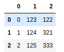
frame = pd.DataFrame(np.arange(4).reshape(2,2)) |

print(frame.to_html()) |
out:
<table border="1" class="dataframe"> |
frame = pd.DataFrame( np.random.random((4,4)), |
in:
s = ['<HTML>'] |
读取
web_frames = pd.read_html('myFrame.html') |
ranking = pd.read_html('http://www.meccanismocomplesso.org/en/ meccanismo-complesso-sito-2/classifica-punteggio/') |
此处省略。。。
ranking[1] |
从XML读取数据
pandas的所有I/O API函数中,没有专门用来处理XML(可扩展标记语言)格式的。虽然没有, 但这种格式其实很重要,因为很多结构化数据都是以XML格式存储的。pandas没有专门的处理函 数也没关系,因为Python有很多读写XML格式数据的库(除了pandas)。
其中一个库叫作lxml,它在大文件处理方面性能优异,因而从众多同类库之中脱颖而出。这 一节将介绍如何用它处理XML文件,以及如何把它和pandas整合起来,以最终从XML文件中获 取到所需数据并将其转换为DataFrame对象。
from lxml import objectify |
root = xml.getroot() |
root.Book.Author |
‘ 272103_l_EnRoss, Mark’
root.Book.PublishDate |
‘2014-22-0l’
mes = root.Book.getchildren() |
[‘ 272103_l_EnRoss, Mark’, ‘XML Cookbook’, ‘Computer’, 23.56, ‘2014-22-0l’]
[child.tag for child in mes] |
[‘Author’, ‘Title’, ‘Genre’, ‘Price’, ‘PublishDate’]
[child.text for child in mes] |
[‘ 272103_l_EnRoss, Mark’, ‘XML Cookbook’, ‘Computer’, ‘23.56’, ‘2014-22-0l’]
读写 Microsoft Excel文件
- to_excel()
- read_excel()
能够读取.xls和.xlsx两种类型的文件
读写JSON数据
- read_json()
- to_json()
HDF5格式
至此,已学习了文本格式的读写。若要分析大量数据,最好使用二进制格式。Python有多 种二进制数据处理工具。HDF5库在这个方面取得了一定的成功。
HDF代表等级数据格式(hierarchical data format )。HDF5库关注的是HDF5文件的读写,这种文件的数据结构由节点组成,能够存储大量数据集。
该库全部用c语言开发,提供了python/matlab和Java语言接口。它的迅速扩展得益于开发人 员的广泛使用,还得益于它的效率,尤其是使用这种格式存储大量数据,其效率很高。比起其他处理起二进制数据更为简单的格式,HDF5支持实时压缩,因而能够利用数据结构中的重复模式压缩文件。
目前,Python提供两种操纵HDF5格式数据的方法:PyTables和h5py。这两种方法有几点不同,选用哪一种很大程度上取决于具体需求。
h5py为HDF5的高级API提供接口。PyTables封装了很多HDF5细节,提供更加灵活的数据容器、索引表、搜索功能和其他计算相关的介质。
pandas还有一个叫作HDFStore、类似于diet的类,它用PyTables存储pandas对象。使用HDF5格式之前,必须导人HDFStore类。
from pandas.io.pytables import HDFStore |
store = HDFStore('mydata.h5') |
store['obj2'] = frame2 |
File path: mydata.h5
store['obj2'] |
store['obj1'] |
pickle ——python对象序列化
pickle模块实现了一个强大的算法,能够对用Python实现的数据结构进行序列化(pickling) 和反序列化操作。序列化是指把对象的层级结构转换为字节流的过程。序列化便于对象的传输、存储和重建,仅用接收器就能重建对象,还能保留它的所有原始特征。
import pickle |
b’\x80\x03}q\x00(X\x05\x00\x00\x00colorq\x01]q\x02(X\x05\x00\x00\x00whiteq\x03X\x03\x00\x00\x00redq\x04eX\x05\x00\x00\x00valueq\x05]q\x06(K\x05K\x07eu.’
nframe = pickle.loads(pickled_data) |
{‘color’: [‘white’, ‘red’], ‘value’: [5, 7]}
用pandas实现对象序列化
用pandas库实现对象序列化(反序列化)很方便,所有工具都是现成的,无需在Python会话中导入cPickle模块,所有的操作都是隐式进行的。 pandas的序列化格式并不是完全使用ASCII编码
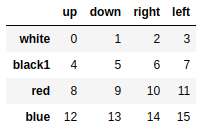
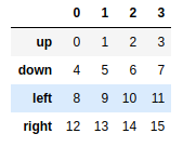
frame = pd.DataFrame(np.arange(16).reshape(4,4), index = ['up','down','left','right']) |
pandas的所有序列化和反序列化操作都在后台运行,用户根本看不到。这使得这两项操作对数据分析人员而言尽可能简单和易于理解。
注意 :使用这种格式时,要确保打开的文件的安全性。pickle格式无法规避错误和恶意数据。
对接数据库
在很多应用中,所使用的数据来自于文本文件的很少,因为文本文件不是存储数据最有效的方式
数据往往存储于SQL类关系型数据库,作为补充,NoSQL数据库近来也已流行开来。
从SQL数据库加载数据,将其转换为DataFrame对象很简单pandas提供的几个函数简化了该过程。
pandas.io.sql模块提供独立于数据库、叫作sqlalchemy的统一接口。该接口简化了连接模式, 不管对于什么类型的数据库,操作命令都只有一套。连接数据库使用create_engine()函数,你可以用它配置驱动器所需的用户名、密码、端口和数据库实例等所有属性。 数据库URL的典型形式是:
dialect+driver://username:password@host:port/database
名称的标识名称,例如sqlite,mysql,postgresql,oracle,或mssql。drivername是用于使用全小写字母连接到数据库的DBAPI的名称。如果未指定,则将导入“默认”DBAPI(如果可用) - 此默认值通常是该后端可用的最广泛的驱动程序。
from sqlalchemy import create_engine |
PostgreSQL
default
engine = create_engine(‘postgresql://scott:tiger@localhost/mydatabase’)
psycopg2
engine = create_engine(‘postgresql+psycopg2://scott:tiger@localhost/mydatabase’)
pg8000
engine = create_engine(‘postgresql+pg8000://scott:tiger@localhost/mydatabase’)
MySql
default
engine = create_engine(‘mysql://scott:tiger@localhost/foo’)
mysql-python
engine = create_engine(‘mysql+mysqldb://scott:tiger@localhost/foo’)
MySQL-connector-python
engine = create_engine(‘mysql+mysqlconnector://scott:tiger@localhost/foo’)
OurSQL
engine = create_engine(‘mysql+oursql://scott:tiger@localhost/foo’)
Oracle
engine = create_engine(‘oracle://scott:tiger@127.0.0.1:1521/sidname’)
engine = create_engine(‘oracle+cx_oracle://scott:tiger@tnsname’)
Microsoft SQL
pyodbc
engine = create_engine(‘mssql+pyodbc://scott:tiger@mydsn’)
pymssql
engine = create_engine(‘mssql+pymssql://scott:tiger@hostname:port/dbname’)
SQLite
由于SQLite连接到本地文件,因此URL格式略有不同。URL的“文件”部分是数据库的文件名。
对于相对文件路径,这需要三个斜杠:
sqlite:///
where is relative:
engine = create_engine(‘sqlite:///foo.db’)
对于绝对文件路径,三个斜杠后面是绝对路径:
Unix/Mac - 4 initial slashes in total
engine = create_engine(‘sqlite:////absolute/path/to/foo.db’)
Windows
engine = create_engine(‘sqlite:///C:\path\to\foo.db’)
Windows alternative using raw string
engine = create_engine(r’sqlite:///C:\path\to\foo.db’)
SQLite3数据读写
学习使用Python内置的SQLite数据库sqlite3。SQLite3工具实现了简单、 轻量级的DBMS SQL,因此可以内置于用Python语言实现的任何应用。它很实用,你可以在单个文件中创建一个嵌入式数据库。
若想使用数据库的所有功能而又不想安装真正的数据库,这个工具就是最佳选择。若想在使用真正的数据库之前练习数据库操作,或在单一程序中使用数据库存储数据而无需考虑接口, SQLite3都是不错的选择。
frame = pd.DataFrame( np.arange(20).reshape(4,5), |
#连接SQLite3数据库 |
数据处理
数据准备
- 加载
- 组装
- 合并(merging)
- 拼接(concatenation)
- 组合(combine)
- 变形(轴向旋转)
- 删除
合并
对于合并操作,熟悉SQL的读者可以将其理解为JOIN操作,它使用一个或多个键把多行数据 结合在一起.
事实上,跟关系型数据库打交道的开发人员通常使用SQL的JOIN查询,用几个表共有的引用 值(键)从不同的表获取数据。以这些键为基础,我们能够获取到列表形式的新数据,这些数据是对几个表中的数据进行组合得到的。pandas库中这类操作叫作合并,执行合并操作的函数为 merge().
import pandas as pd |
frame2 = pd.DataFrame( {'id':['pencil','pencil','ball','pen'], |
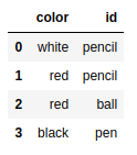
pd.merge(frame1,frame2) |
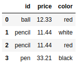
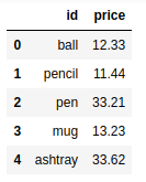
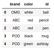
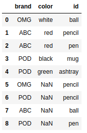
frame1 = pd.DataFrame( {'id':['ball','pencil','pen','mug','ashtray'], |
frame2 = pd.DataFrame( {'id':['pencil','pencil','ball','pen'], |
pd.merge(frame1,frame2) |
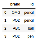
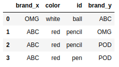
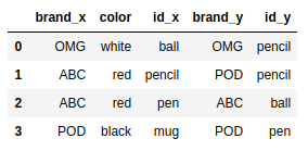
pd.merge(frame1,frame2,on='id') |
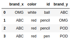
pd.merge(frame1,frame2,on='brand') |
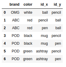
假如两个DataFrame基准列的名称不一致,该怎样进行合并呢?为 了解决这个问题,你可以用left_on和right_on选项指定第一个和第二个DataFrame的基准列。
frame2.columns = ['brand','sid'] |
pd.merge(frame1,frame2,left_on='id',right_on='sid') |
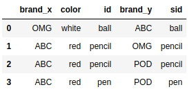
merge()函数默认执行的是内连接操作;上述结果中的键是由交叉操作(intersection)得到的。
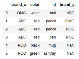
其他选项有左连接、右连接和外连接。外连接把所有的键整合到一起,其效果相当于左连接 和右连接的效果之和。连接类型用how选项指定。
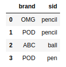
frame2.columns = ['brand','id'] |
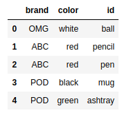
frame4 = pd.DataFrame( {'id':['ball','pencil','pen','mug','ashtray'], |
pd.merge(frame4,frame2,on='id') |
pd.merge(frame4,frame2,on='id',how='outer') |
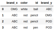
pd.merge(frame4,frame2,on='id',how='left') |
pd.merge(frame4,frame2,on='id',how='right') |
pd.merge(frame4,frame2,on=['id','brand'],how='outer') |
根据索引合并
pd.merge(frame4,frame2,right_index=True, left_index=True) |
#frame4.join(frame2) #会报错,因为列名有重合 |
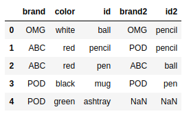
frame2.columns = ['brand2','id2'] |
frame4.join(frame2) |
拼接
另外一种数据整合操作叫作拼接(concatenation)。NumPy的concatenate()函数就是用于数 组的拼接操作。
array1 = np.arange(9).reshape((3,3)) |
array([[0, 1, 2],
[3, 4, 5],
[6, 7, 8]])
array2 = np.arange(9).reshape((3,3))+6 |
array([[ 6, 7, 8],
[ 9, 10, 11],
[12, 13, 14]])
np.concatenate([array1,array2],axis = 1) |
array([[ 0, 1, 2, 6, 7, 8],
[ 3, 4, 5, 9, 10, 11],
[ 6, 7, 8, 12, 13, 14]])
np.concatenate([array1,array2],axis = 0) |
array([[ 0, 1, 2],
[ 3, 4, 5],
[ 6, 7, 8],
[ 6, 7, 8],
[ 9, 10, 11],
[12, 13, 14]])
pandas库以及它的Series和DataFrame等数据结构实现了带编号的轴,它可以进一步扩展数组
拼接功能。pandas的concat()函数实现了按轴拼接的功能。
ser1 = pd.Series(np.random.rand(4),index=[1,2,3,4]) |
1 0.676614
2 0.607490
3 0.491370
4 0.687731
dtype: float64
ser2 = pd.Series(np.random.rand(4),index=[5,6,7,8]) |
5 0.129962
6 0.650653
7 0.701635
8 0.820312
dtype: float64
pd.concat([ser1,ser2]) |
1 0.676614
2 0.607490
3 0.491370
4 0.687731
5 0.129962
6 0.650653
7 0.701635
8 0.820312
dtype: float64
concat()函数默认按照axis=0这条轴拼接数据,返回Series对象。如果指定axis=l,返回结果将是DataFrame对象。
pd.concat([ser1,ser2],axis=1) |

pd.concat([ser1,ser2],keys=[1,2]) #等级索引 |
1 1 0.676614
2 0.607490
3 0.491370
4 0.687731
2 5 0.129962
6 0.650653
7 0.701635
8 0.820312
dtype: float64
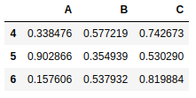
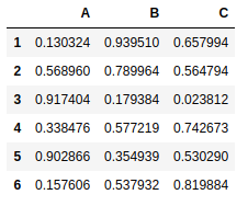
frame5 = pd.DataFrame(np.random.rand(9).reshape(3,3), index=[1,2,3],columns=['A','B','C']) |
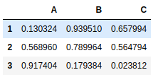
frame2 = pd.DataFrame(np.random.rand(9).reshape(3,3), index=[4,5,6],columns=['A','B','C']) |
pd.concat([frame5,frame2]) |
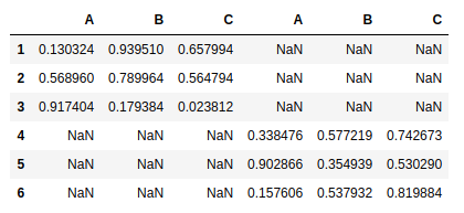
pd.concat([frame5,frame2],axis = 1) |
组合
还有另外一种情况,我们无法通过合并或拼接方法组合数据。例如,两个数据集的索引完全或部分重合。
ser1 = pd.Series(np.random.rand(5),index=[1,2,3,4,5]) |
1 0.479704
2 0.956898
3 0.785966
4 0.868556
5 0.134064
dtype: float64
ser2 = pd.Series(np.random.rand(4),index=[2,4,5,6]) |
2 0.337220
4 0.570806
5 0.419785
6 0.140270
dtype: float64
ser1.combine_first(ser2) |
1 0.479704
2 0.956898
3 0.785966
4 0.868556
5 0.134064
6 0.140270
dtype: float64
ser2.combine_first(ser1) |
1 0.479704
2 0.337220
3 0.785966
4 0.570806
5 0.419785
6 0.140270
dtype: float64
ser1[:3].combine_first(ser2[:3]) |
1 0.479704
2 0.956898
3 0.785966
4 0.570806
5 0.419785
dtype: float64
轴向旋转
frame5 = pd.DataFrame(np.arange(9).reshape(3,3), |
out:
ball pen pencil |
in:
frame6 = frame5.stack() #列变行 |
out:
white ball 0 |
in:
frame6.unstack() |
frame6.unstack(0) |

in:
frame5.unstack() |
out:
ball white 0 |
in:
longframe = pd.DataFrame({ 'color':['white','white','white','red','red','red','black','black','black'], |
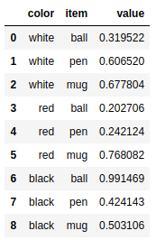
这种记录数据的模式有几个缺点。例如其中一个缺点是,因为一些字段具有多样性和 重复性特点,所以选取列作为键时,这种格式的数据可读性较差,尤其是无法完全理解基准列和 其他列之间的关系a
除了长格式,还有一种把数据调整为表格形式的宽格式。这种模式可读性强,也易于连接其他表,且占用空间较少。因此一般而言,用它存储数据效率更高,虽然它的可操作性差,这一点 尤其体现在填充数据时。
如要选择一列或几列作为主键,所要遵循的规则是其中的元素必须是唯一的。
讲到格式转换,pandas提供了能够把长格式DataFrame转换为宽格式的pivot()函数,它以用 作键的一列或多列作为参数。
接着上面的例子,选择color列作为主键,item列作为第二主键,而它们所对应的元素则作 为DataFrame的新列。
wideframe = longframe.pivot('color','item') |
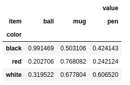
这种格式的DataFrame对象更加紧凑,它里面的数据可读性也更强。
删除
数据处理的最后一步是删除多余的行和列。
frame7 = pd.DataFrame(np.arange(9).reshape(3,3), |
del frame7['ball'] #删除列 |
frame7.drop('white') #删除行 |
frame7.drop('pen',axis=1) |
数据转换
删除重复元素
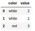
dframe = pd.DataFrame({ 'color': ['white','white','red','red','white'],'value': [2,1,3,3,2]}) |
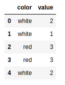
DataFrame对象的duplicated()函数可用来检测重复的行,返回元素为布尔型的Series对象。 每个元素对应一行,如果该行与其他行重复(也就是说该行不是第一次出现),则元素为True; 如果跟前面不重复,则元素就为False。
dframe.duplicated() |
0 False
1 False
2 False
3 True
4 True
dtype: bool
返回元素为布尔值的Series对象用处很大,特别适用于过滤操作。
dframe[dframe.duplicated()] |
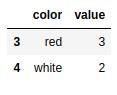
通常,所有重复的行都需要从DataFrame对象中删除。pandas库的drop_duplicates()函数实
现了删除功能,该函数返回的是删除重复行后的DataFmme对象。
dframe.drop_duplicates() |
映射
用映射替换元素
frame8 = pd.DataFrame({ 'item':['ball','mug','pen','pencil','ashtray'], |
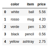
要用新元素替换不正确的元素,需要定义一组映射关系。在映射关系中,旧元素作为键,新元素作为值。
newcolors ={ |
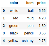
DataFrame对象中两种旧颜色被替换为正确的元素。还有一种常见情况,是把NaN替换为其他值,比如0。这种情况下,仍然可以用replace()函数,它能优雅地完成该项操作。
ser = pd.Series([13,np.nan,4,6,np.nan,3]) |
0 13.0
1 NaN
2 4.0
3 6.0
4 NaN
5 3.0
dtype: float64
ser.replace(np.nan,0) |
0 13.0
1 0.0
2 4.0
3 6.0
4 0.0
5 3.0
dtype: float64
用映射添加元素
frame9 = pd.DataFrame({ 'item':['ball','mug','pen','pencil','ashtray'], 'color':['white','red','green','black','yellow']}) |
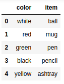
price = { |
frame9['price'] = frame9['item'].map(price) |
重命名轴索引
reindex = { |
recolumn ={ |
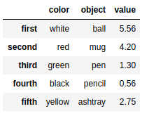
索引被重命名。若要重命名各列,必须使用columns选项
frame9.rename(index = reindex,columns=recolumn) |
对于只有单个元素要替换的最简单情况,可以对传入的参数做进一步限定,而无需把多个变 量都写出来,也避免产生多次赋值操作。
frame9.rename(index={1:'first'},columns = {'item':'object'}) |
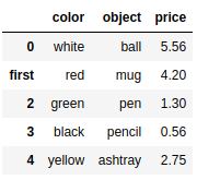
frame9 |
frame9.rename(index={1:'first'},columns = {'item':'object'},inplace=True) |
frame9 |
离散化和面元划分
ages=[20,22,25,27,21,23,37,31,61,45,41,32] |
cat = pd.cut(ages,bins) |
out:
[(18, 25], (18, 25], (18, 25], (25, 35], (18, 25], ..., (25, 35], (60, 100], (35, 60], (35, 60], (25, 35]] |
in:
cat.codes |
array([0, 0, 0, 1, 0, 0, 2, 1, 3, 2, 2, 1], dtype=int8)
每个面元的出现次数,即每个类别有多少个元素,可使用value_counts()函数。
pd.value_counts(cat) ##查看每个种类的数量 |
(18, 25] 5
(35, 60] 3
(25, 35] 3
(60, 100] 1
dtype: int64
cuts = pd.cut(ages,bins,right=False) ## 使用right=False可以修改开端和闭端 |
out:
[[18, 25), [18, 25), [25, 35), [25, 35), [18, 25), ..., [25, 35), [60, 100), [35, 60), [35, 60), [25, 35)] |
in:
cut1 = pd.cut(ages,bins,right=False,labels=list('abcd')) |
out:
[a, a, b, b, a, ..., b, d, c, c, b] |
in:
pd.cut(ages,5) # 如果cut传入的是数字n,那么就会均分成n份。 |
out:
[(19.959, 28.2], (19.959, 28.2], (19.959, 28.2], (19.959, 28.2], (19.959, 28.2], ..., (28.2, 36.4], (52.8, 61.0], (44.6, 52.8], (36.4, 44.6], (28.2, 36.4]] |
pd.value_counts(pd.cut(ages,4)) |
(19.959, 30.25] 6
(30.25, 40.5] 3
(40.5, 50.75] 2
(50.75, 61.0] 1
dtype: int64
pd.qcut(ages,5) |
out:
[(19.999, 22.2], (19.999, 22.2], (22.2, 25.8], (25.8, 31.6], (19.999, 22.2], ..., (25.8, 31.6], (40.2, 61.0], (40.2, 61.0], (40.2, 61.0], (31.6, 40.2]] |
in:
pd.value_counts(pd.qcut(ages,4)) |
out:
(38.0, 61.0] 3 |
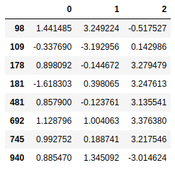
异常值检测和过滤
data = pd.DataFrame(np.random.randn(1000,3)) |
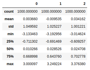
可能会将比标准差大3倍的元素视作异常值。用std()函数就可以求得DataFrame对象每一列的标准差。
3σ原则
data.std() |
0 1.049592
1 1.025227
2 1.001221
dtype: float64
data[(np.abs(data-data.mean())>(3*data.std())).any(1)] #过滤条件 |
排序
nframe = pd.DataFrame(np.arange(25).reshape(5,5)) |
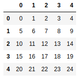
new_order = np.random.permutation(5) #乱序整数[0-4] 如果是100 [0-99] |
array([4, 0, 3, 1, 2])
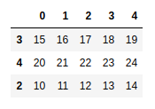
nframe.take(new_order) #排序 |
np.random.permutation(100) |
out:
array([94, 5, 24, 55, 99, 80, 76, 25, 82, 66, 52, 37, 87, 16, 15, 78, 69, |
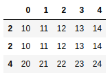
nframe.take([3,4,2]) #只对一部分排序 |
sample = np.random.randint(len(nframe),size =3) #随机整数 |
array([2, 2, 4])
nframe.take(sample) |
数据聚合
GroupBy
frame10 = pd.DataFrame({ 'color': ['white','red','green','red','green'],'object': ['pen','pencil','pencil','ashtray','pen'], |
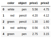
group = frame10['price1'].groupby(frame10['color']) |
group.groups |
{‘green’: Int64Index([2, 4], dtype=’int64’),
‘red’: Int64Index([1, 3], dtype=’int64’),
‘white’: Int64Index([0], dtype=’int64’)}
group.sum() |
color
green 4.05
red 4.76
white 5.56
Name: price1, dtype: float64
group.mean() |
color
green 2.025
red 2.380
white 5.560
Name: price1, dtype: float64
等级分组
ggroup = frame10['price1'].groupby([frame10['color'],frame10['object']]) |
ggroup.groups |
{(‘green’, ‘pen’): Int64Index([4], dtype=’int64’),
(‘green’, ‘pencil’): Int64Index([2], dtype=’int64’),
(‘red’, ‘ashtray’): Int64Index([3], dtype=’int64’),
(‘red’, ‘pencil’): Int64Index([1], dtype=’int64’),
(‘white’, ‘pen’): Int64Index([0], dtype=’int64’)}
ggroup.sum() |
out:
color object |
in:
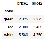
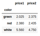
frame10[['price1','price2']].groupby(frame10['color']).mean() |
组迭代
for name,group in frame10.groupby('color'): |
out:
green |
链式转换
result1 = frame10['price1'].groupby(frame10['color']).mean() |
color
green 2.025
red 2.380
white 5.560
Name: price1, dtype: float64
result2 = frame10.groupby(frame10['color']).mean() |
frame10.groupby(frame10['color'])['price1'].mean() |
color
green 2.025
red 2.380
white 5.560
Name: price1, dtype: float64
(frame10.groupby(frame10['color']).mean())['price1'] |
color
green 2.025
red 2.380
white 5.560
Name: price1, dtype: float64
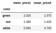
frame10.groupby('color').mean().add_prefix('mean_') |
替换
maps = {'x':xx} |
取值
sub_data = data.loc[data['name']==1] |