支持向量机（SVM）

import numpy as np
import matplotlib.pyplot as plt
from scipy import stats

# use seaborn plotting defaults
import seaborn as sns; sns.set()
%matplotlib inline

支持向量基本原理

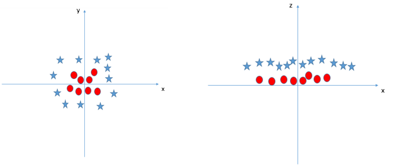
如何解决这个线性不可分问题呢？咱们给它映射到高维来试试

$z=x^2+y^2$

例子

#随机来点数据
from sklearn.datasets.samples_generator import make_blobs  #制造数据集
X, y = make_blobs(n_samples=50, centers=2,
                  random_state=0, cluster_std=0.60)        #cluster_std 离散程度

print(X.shape)
print(y.shape)
plt.scatter(X[:, 0], X[:, 1], c=y, s=50, cmap='autumn')    #https://matplotlib.org/tutorials/colors/colormaps.html  s 大小

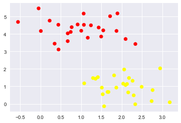
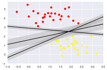
随便的画几条分割线，哪个好来着？

xfit = np.linspace(-1, 3.5)
plt.scatter(X[:, 0], X[:, 1], c=y, s=50, cmap='autumn')
plt.plot([0.6], [2.1], 'x', color='red', markeredgewidth=2, markersize=10)

for m, b in [(1, 0.65), (0.5, 1.6), (-0.2, 2.9)]:
    plt.plot(xfit, m * xfit + b, '-k')

plt.xlim(-1, 3.5);

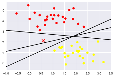
Support Vector Machines: 最小化雷区

xfit = np.linspace(-1, 3.5)
plt.scatter(X[:, 0], X[:, 1], c=y, s=50, cmap='autumn')

for m, b, d in [(1, 0.65, 0.33), (0.5, 1.6, 0.55), (-0.2, 2.9, 0.2)]:
    yfit = m * xfit + b
    plt.plot(xfit, yfit, '-k')
    plt.fill_between(xfit, yfit - d, yfit + d, edgecolor='none',
                     color='#AAAAAA', alpha=0.4)

plt.xlim(-1, 3.5);

训练一个基本的SVM

from sklearn.svm import SVC # "Support vector classifier"
model = SVC(kernel='linear')
model.fit(X, y)

SVC(C=1.0, cache_size=200, class_weight=None, coef0=0.0,
  decision_function_shape='ovr', degree=3, gamma='auto', kernel='linear',
  max_iter=-1, probability=False, random_state=None, shrinking=True,
  tol=0.001, verbose=False)

#绘图函数
def plot_svc_decision_function(model, ax=None, plot_support=True):
    """Plot the decision function for a 2D SVC"""
    if ax is None:
        ax = plt.gca() #创建一个实例
    xlim = ax.get_xlim() #获取x轴范围
    ylim = ax.get_ylim() #获取y轴范围
    
    # create grid to evaluate model
    x = np.linspace(xlim[0], xlim[1], 30) 
    y = np.linspace(ylim[0], ylim[1], 30)
    

    Y, X = np.meshgrid(y, x)     #从坐标向量返回坐标矩阵
    xy = np.vstack([X.ravel(), Y.ravel()]).T    #连续的扁平数组    #垂直堆叠数组（行方式）  2列
    P = model.decision_function(xy).reshape(X.shape)  #xy到分离超平面的距离
    
    # plot decision boundary and margins
    ax.contour(X, Y, P, colors='k', 
               levels=[-1, 0, 1], alpha=0.5,
               linestyles=['--', '-', '--'])   #等高线绘图和标注的类。
    
    # plot support vectors
    if plot_support:
        ax.scatter(model.support_vectors_[:, 0],
                   model.support_vectors_[:, 1],
                   s=300, linewidth=1, facecolors='none');
    ax.set_xlim(xlim)
    ax.set_ylim(ylim)

plt.scatter(X[:, 0], X[:, 1], c=y, s=50, cmap='autumn')
plot_svc_decision_function(model);

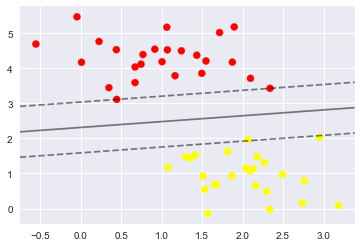
这条线就是我们希望得到的决策边界啦
观察发现有3个点做了特殊的标记，它们恰好都是边界上的点
它们就是我们的support vectors（支持向量）
在Scikit-Learn中, 它们存储在这个位置 support_vectors_（一个属性）

model.support_vectors_

array([[0.44359863, 3.11530945],
[2.33812285, 3.43116792],
[2.06156753, 1.96918596]])

观察可以发现，只需要支持向量我们就可以把模型构建出来
接下来我们尝试一下，用不同多的数据点，看看效果会不会发生变化
分别使用60个和120个数据点

def plot_svm(N=10, ax=None):
    X, y = make_blobs(n_samples=200, centers=2,
                      random_state=0, cluster_std=0.60)
    X = X[:N]
    y = y[:N]
    model = SVC(kernel='linear', C=1E10)
    model.fit(X, y)
    
    ax = ax or plt.gca()
    ax.scatter(X[:, 0], X[:, 1], c=y, s=50, cmap='autumn')
    ax.set_xlim(-1, 4)
    ax.set_ylim(-1, 6)
    plot_svc_decision_function(model, ax)

fig, ax = plt.subplots(1, 2, figsize=(16, 6))
fig.subplots_adjust(left=0.0625, right=0.95, wspace=0.1)
for axi, N in zip(ax, [60, 120]):
    plot_svm(N, axi)
    axi.set_title('N = {0}'.format(N))

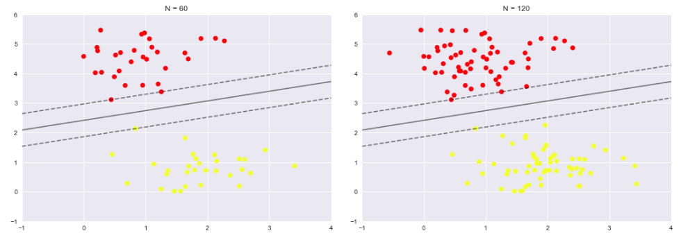
左边是60个点的结果，右边的是120个点的结果
观察发现，只要支持向量没变，其他的数据怎么加无所谓！

引入核函数的SVM

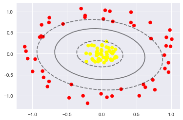
首先我们先用线性的核来看一下在下面这样比较难的数据集上还能分了吗？

from sklearn.datasets.samples_generator import make_circles
X, y = make_circles(100, factor=.1, noise=.1)

clf = SVC(kernel='linear').fit(X, y)

plt.scatter(X[:, 0], X[:, 1], c=y, s=50, cmap='autumn')
plot_svc_decision_function(clf, plot_support=False);

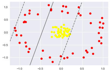
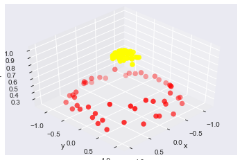
坏菜喽，分不了了，那咋办呢？试试高维核变换吧！

We can visualize this extra data dimension using a three-dimensional plot:

#加入了新的维度r
from mpl_toolkits import mplot3d
r = np.exp(-(X ** 2).sum(1))
def plot_3D(elev=30, azim=30, X=X, y=y):
    ax = plt.subplot(projection='3d')
    ax.scatter3D(X[:, 0], X[:, 1], r, c=y, s=50, cmap='autumn')
    ax.view_init(elev=elev, azim=azim)
    ax.set_xlabel('x')
    ax.set_ylabel('y')
    ax.set_zlabel('r')

plot_3D(elev=45, azim=45, X=X, y=y)

#加入基函数
clf = SVC(kernel='rbf', C=1E6)
clf.fit(X, y)

SVC(C=1000000.0, cache_size=200, class_weight=None, coef0=0.0,
decision_function_shape=’ovr’, degree=3, gamma=’auto’, kernel=’rbf’,
max_iter=-1, probability=False, random_state=None, shrinking=True,
tol=0.001, verbose=False)

plt.scatter(X[:, 0], X[:, 1], c=y, s=50, cmap='autumn')
plot_svc_decision_function(clf)
plt.scatter(clf.support_vectors_[:, 0], clf.support_vectors_[:, 1],
            s=300, lw=1, facecolors='none');

使用这种核支持向量机，我们学习一个合适的非线性决策边界。这种核变换策略在机器学习中经常被使用！

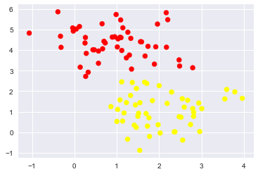
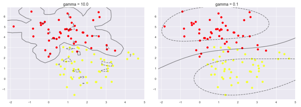
调节SVM参数: Soft Margin问题

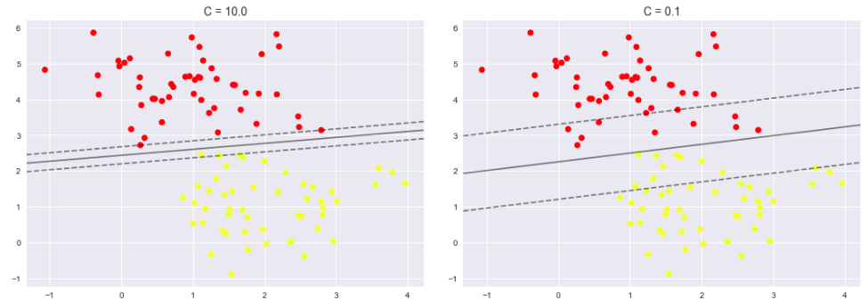
调节C参数

当C趋近于无穷大时：意味着分类严格不能有错误
当C趋近于很小的时：意味着可以有更大的错误容忍

X, y = make_blobs(n_samples=100, centers=2,
                  random_state=0, cluster_std=0.8)
plt.scatter(X[:, 0], X[:, 1], c=y, s=50, cmap='autumn');

X, y = make_blobs(n_samples=100, centers=2,
                  random_state=0, cluster_std=0.8)

fig, ax = plt.subplots(1, 2, figsize=(16, 6))
fig.subplots_adjust(left=0.0625, right=0.95, wspace=0.1)

for axi, C in zip(ax, [10.0, 0.1]):
    model = SVC(kernel='linear', C=C).fit(X, y)
    axi.scatter(X[:, 0], X[:, 1], c=y, s=50, cmap='autumn')
    plot_svc_decision_function(model, axi)
    axi.scatter(model.support_vectors_[:, 0],
                model.support_vectors_[:, 1],
                s=300, lw=1, facecolors='none');
    axi.set_title('C = {0:.1f}'.format(C), size=14)

X, y = make_blobs(n_samples=100, centers=2,
                  random_state=0, cluster_std=1.1)

fig, ax = plt.subplots(1, 2, figsize=(16, 6))
fig.subplots_adjust(left=0.0625, right=0.95, wspace=0.1)

for axi, gamma in zip(ax, [10.0, 0.1]):
    model = SVC(kernel='rbf', gamma=gamma).fit(X, y)        #gamma越大越复杂，gamma越小越简单
    axi.scatter(X[:, 0], X[:, 1], c=y, s=50, cmap='autumn')
    plot_svc_decision_function(model, axi)
    axi.scatter(model.support_vectors_[:, 0],
                model.support_vectors_[:, 1],
                s=300, lw=1, facecolors='none');
    axi.set_title('gamma = {0:.1f}'.format(gamma), size=14)

Example: Face Recognition

面部识别

from sklearn.datasets import fetch_lfw_people
faces = fetch_lfw_people(min_faces_per_person=60)
print(faces.target_names)
print(faces.images.shape)

[‘Ariel Sharon’ ‘Colin Powell’ ‘Donald Rumsfeld’ ‘George W Bush’
‘Gerhard Schroeder’ ‘Hugo Chavez’ ‘Junichiro Koizumi’ ‘Tony Blair’]
(1348, 62, 47)

Let’s plot a few of these faces to see what we’re working with:

fig, ax = plt.subplots(3, 5)

fig.tight_layout()

for i, axi in enumerate(ax.flat):
    
    axi.imshow(faces.images[i],cmap='bone' )   #黑白 
    axi.set(xticks=[], yticks=[],
            xlabel=faces.target_names[faces.target[i]])

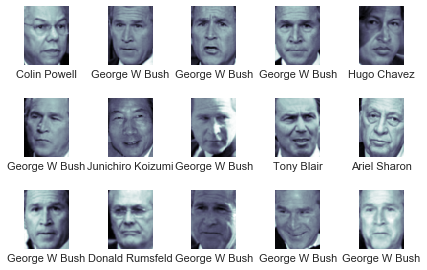
每个图的大小是 [62×47]
在这里我们就把每一个像素点当成了一个特征，但是这样特征太多了，用PCA降维一下吧！

from sklearn.svm import SVC
#from sklearn.decomposition import RandomizedPCA
from sklearn.decomposition import PCA
from sklearn.pipeline import Pipeline

from sklearn.model_selection import train_test_split
Xtrain, Xtest, ytrain, ytest = train_test_split(faces.data, faces.target,
                                                random_state=40)

使用grid search cross-validation来选择我们的参数

from sklearn.model_selection import GridSearchCV
param_grid = {'svc__C': [1, 5, 10],
              'svc__gamma': [0.0001, 0.0005, 0.001]}

pipe = Pipeline([

            ('pca',PCA(n_components = 150 ,whiten=True, random_state=64)),
            ('svc', SVC(kernel='rbf', class_weight='balanced'))
        ])

grid = GridSearchCV(pipe, param_grid)
grid.fit(Xtrain,ytrain)
print(grid.best_params_)

{‘svcC’: 5, ‘svcgamma’: 0.001}

model = grid.best_estimator_
yfit = model.predict(Xtest)
yfit.shape

(337,)

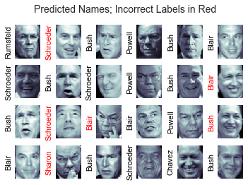
看看咋样吧！

fig, ax = plt.subplots(4, 6)
for i, axi in enumerate(ax.flat):
    axi.imshow(Xtest[i].reshape(62, 47), cmap='bone')
    axi.set(xticks=[], yticks=[])
    axi.set_ylabel(faces.target_names[yfit[i]].split()[-1],
                   color='black' if yfit[i] == ytest[i] else 'red')
fig.suptitle('Predicted Names; Incorrect Labels in Red', size=14);

from sklearn.metrics import classification_report
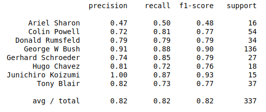
print(classification_report(ytest, yfit,
                            target_names=faces.target_names))

精度(precision) = 正确预测的个数(TP)/被预测正确的个数(TP+FP)
召回率(recall)=正确预测的个数(TP)/预测个数(TP+FN)
F1 = 2精度召回率/(精度+召回率)

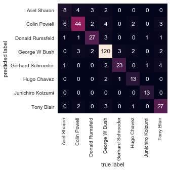
from sklearn.metrics import confusion_matrix
mat = confusion_matrix(ytest, yfit)
sns.heatmap(mat.T, square=True, annot=True, fmt='d', cbar=False,
            xticklabels=faces.target_names,
            yticklabels=faces.target_names)
plt.xlabel('true label')
plt.ylabel('predicted label');